EMC VNX – RAID groups vs Storage Pools
With EMC training I have learnt some general guidelines, that should be followed to optimize and enable good performance on a VNX Unified storage system.
Drive types
When you chose a specific drive type, you should base your choice upon the expected workload.
- FLASH – Extreme Performance Tier – great for extreme performance.
- SAS – Performance Tier – perfect for general performance. Usually 10k RPM or 15k RPM.
- NL-SAS – Capacity Tier – most cost effective, for streaming, agining data and archives and backups
RAID groups
When we want to provision storage on our hard drives, first we have to create either a RAID group, or a Storage Pool. Let’s first review RAID groups.
RAID Levels
Within EMC VNX RAID groups should have a maximum count of 16 drives (which is strange, since this rule does not apply to NetApp at all!).
Choosing the correct drive type is only one step, you also have to choose a correct RAID group.
- RAID 1/0 – this RAID group is appropriate for heavy transactional workloads with a high rate of random writes (let’s say greater than 25-30%)
- RAID 5 – I would say this one is most common one. Works best for medium to high performance, general-purpose and sequential workloads. And it’s much more space effective, since blocks are not mirrored, and parity takes only one extra disk (distributed on all disks thru the RAID group)
- RAID 6 – Most often used for NL-SAS. Works best with read-based workloads such as archiving and backup to disk. It provides additional RAID protection (two disk may fail in one RAID group, instead of 1 with RAID5).
As I mentioned before, RAID groups can have a maximum count of 16 drives (not with NetApp). For parity RAID, the higher the count, the higher the capacity utilization (since there is only one parity disk in RAID5, and 2 parity disks in RAID6 regardless the RAID group size).
Preffered RAID configuration
With a predominance of large-block sequential operations the following rules are most effective:
- RAID5 has a preference of 4+1 or 8+1
- RAID6 has a preference of 8+2 or 14+2
- RAID1/0 has a preference of 4+4
One more tip – when creating RAID groups, select drives from the same bus if possible to boost performance (always prefer horizontal over vertical selection).
Storage Pools
A storage pool is somehow analogous to a RAID group. In few words it’s a physical collection of disks on which logical units (LUNs) are created. Pools are dedicated for use by pool (thin or thick) LUNs. Where RAID group can only contain up to 16 disks, pool can contain hundreds of disks. Because of that, pool-based provisioning spreads workloads over many resources requiring minimal planning and management effort.
Of course pool has the same level of protection against disk failure as RAID groups, simply because RAID groups are used to build up pool. In fact, during pool creation, you have to choose which RAID configuration you preffer.
Pools can be homogeneous or heterogeneous. Homogeneous pools have a single drive type (e.g. SAS or NL-SAS) whereas heterogenous pools contain different drive types. Why EMC allow us to mix different drive types in one pool? Actually it’s pretty clever, le me go a little deeper into that:
Homogeneous pools
Pools with single drive type are recommended for application with similar and expected performance requirements. Only one drive (Flash, SAS, NL-SAS) is available for selection during pool creation.
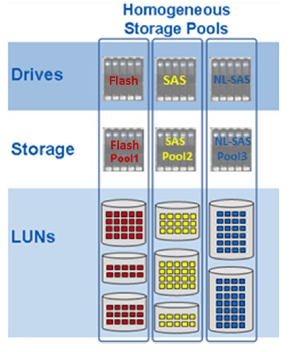
Homogeneous Storage Pools
Picture above shows three Storage pools, one created from Flash Drives (extreme performance tier), another created form SAS drives (performance tier) and the third one created from NL-SAS drives (capacity tier)
Heterogeneous pools
As mentioned previously, heterogeneous pools can consist different types of drives. VNX supports Flash, SAS, and NL-SAS drives in one pool. Heterogeneous pools provide the infrastructure for FAST VP (Fully Automated Storage Tiering for Virtual Pools).
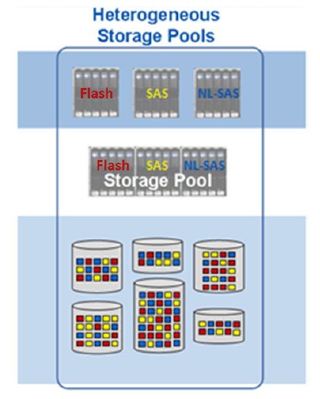
Heterogeneous Storage Pools
FAST VP facilitates automatic data movement to appropriate drive tiers depending on the I/O activity for that data. The most frequently accessed data is moved to the highest tier (Flash drives) in the pool for faster access. Medium activity data is moved to SAS drives, and low activity data is moved to the lowest tier (NL-SAS drives).